Hybrid Quantum Neural Networks for Image Classification

Project Overview

Sample vehicles labled with their make, model and year taken from the VMMRdb dataset

As we reach limits with classical compute power, it becomes necessary to investigate methods that execute faster and are capable of solving more difficult problems. By applying concepts from quantum mechanics to the computing space, we can leverage the power of superposition, entanglement, and interference to parallelize operations and operate at higher dimensions.

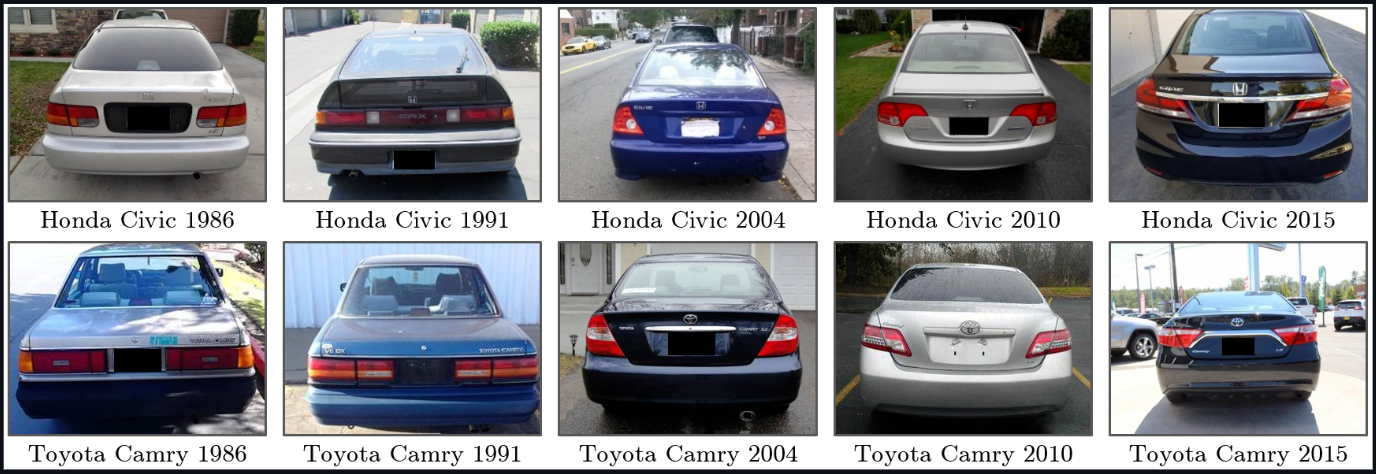
In this project, we compare classical machine learning with quantum machine learning through image-based car model classification algorithms. Specifically, our models predict vehicle make, model and year. This problem being chosen because it's already sufficiently difficult for a classic approach using convolutional neural networks due to the minute level of detail a model would need to extract to differentiate between model years. Our goal with this project is to determine whether quantum-enhanced models can achieve performance comparable to or superior to classical approaches in the context of image classification.

We explored two separate approaches:

A smaller-scale experiment comparing a classical CNN against a hybrid quantum model using a quanvolutional preprocessing layer.
A larger-scale experiment using a ResNet-50 backbone combined with a variational quantum circuit head training on a combined Stanford Cars and VMMRdb dataset

Datasets

Stanford Cars Dataset

The Stanford Cars dataset contains 16,185 images across 196 vehicle classes. Each class generally represents a specific vehicle make, model and year combination.

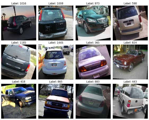
VMMRdb Dataset

The vehicle Make and Model Recognition Database (VMMRdb) contains 291,752 images across 9,170 classes. The dataset includes variation in lighting conditions, image quality, and camera angle. Though generally the same angles are used across classes.

Dataset Processing

This normalization was done solely on the larger-scale normalization. The smaller-scale explored 3-10 classes in the Stanford Cars dataset, so this normalization wasn't necessary.

Normalized class labels across both datasets.
Removed trim, body style and other identifiers that weren't considered make, or model in order to align overlapping classes
Filtered out classes with fewer than 40 images
Limited each class to a maximum of 100 images per dataset to reduce imbalance.
Our final combined dataset contained 2023 classes

Data Augmentation

This was generally identical across both experiments. We even explored the impact of RGB channel normalization in the small experiment. All of this augmentation was in an effort to decrease the chance of overfitting, improve convergence, and create a more robust dataset.

Resized images to 224 x 224
Added random horizontal flips
Added random color jitter
Added random rotation
Added RGB channel normalization

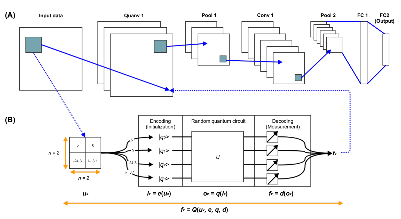
Grid of cars showing augmentation: color jitter, slight rotation and more

Quanvolutional Layer Architecture

The operation of the quanvolutional layer follows a pipeline similar to that of a classical convolution. A small subsection of the image, denoted as u_x, is first selected from the input image. This local subsection may be, for example, a 2×2 or 3×3 patch of pixels. The values in this patch are then encoded into a quantum state through an encoding function e, producing an initialized quantum state i_x = e(u_x). After encoding, the quantum state is processed by a quantum circuit q, producing an output quantum state o_x = q(i_x). Finally, the information contained in this output quantum state is decoded back into a classical scalar value through a decoding function d, yielding the final quanvolutional feature value f_x = d(o_x). This transformation can be summarized as f_x = Q(u_x, e, q, d), where Q represents the full quanvolutional filter transformation.

Conceptually, the quanvolutional layer attempts to use the high-dimensional structure of quantum mechanics to generate feature transformations that may be difficult to reproduce classically. In the same way that classical convolutional filters detect local image patterns, the quantum circuits act as feature detectors operating on local image regions. However, instead of simple matrix multiplications and additions, the local data undergoes a quantum evolution through entangling gate operations and quantum superposition. In our implementation, we specifically use random quantum circuits for these transformations in order to establish a baseline implementation of the architecture. An important aspect of the quanvolutional approach is that the quantum circuits operate only on small local regions of the image rather than on the entire image at once. This design choice significantly reduces the required quantum resources. Because each local patch contains only a small number of pixels, only a small number of qubits are needed per quantum filter. This makes the approach potentially suitable for noisy intermediate-scale quantum (NISQ) hardware, since the circuits can remain relatively shallow and require little or no error correction.

Combined Dataset Architecture

Classical Baseline ResNet-50 Model

We used a ResNet-50 convolutional neural network as the classical baseline. At their core, ResNet architectures utilize residual connections to improve gradient flow, which enables deeper networks while mitigating the vanishing gradient problem. To improve computational efficiency, ResNet models also use bottleneck blocks that intentionally reduce channel dimensionality before doing to bulk of the convolution computation.

Hybrid Quantum Neural Network (HQNN)

Our hybrid architecture combines a pretrained ResNet-50 backbone with a variational quantum circuit implemented using PennyLane. The ResNet-50 acts as a feature extractor, producing a 2048-dimensional feature vector that is then projected down to the number of qubits our circuit uses. That number being 6 in our case. Those 6 features are then encoded into the quantum circuit through parameterized rotation gates and then mapped back into the classical feature space to produce the final classification outputs.

Results

Combined Dataset

ResNet-50 Top-1 Accuracy

35.78%

ResNet-50 Top-5 Accuracy

65.50%

HQNN Top-1 Accuracy

0.21%

HQNN Top-5 Accuracy

0.81%

The classical ResNet-50 model significantly outperformed the hybrid HQNN on the large-scale dataset. Fine-tuninng of a pretrained ResNet-50 model with our quantum circuit head was tried with minimal gain, only a 0.41% improvement above an HQNN model not using fine-tuning. Overall, the projection from a 2048 feature space down to a 6 dimentional feature space is likely the cause of this drop in performance. In our future work we consider some ideas of how to potentially improve this.

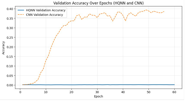
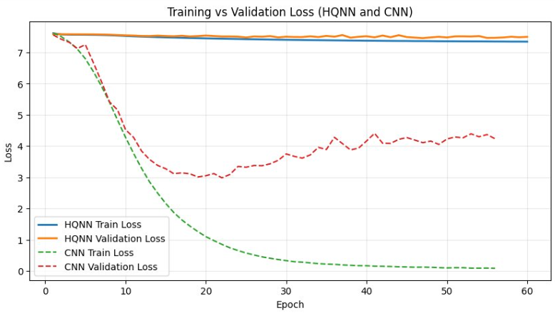
CNN and HQNN Validation Accuracy over Epochs

CNN and HQNN Validation Loss over Epochs

The validation accuracy, validation loss, and training loss remains constant while training the HQNN, not improving much at all. The validation accuracy, validation loss and training loss for the CNN/ResNet-50 model do improve for around 20 epochs before the model actually begins to overfit as shown by the increase in validation loss and the jitteriness of the validation accuracy after that point.

Subset Results

With the simulation for a QNN on a small subset of data, it was evident that adding the quanvolutional layer had noticeable improvements over a solely classical implementation. However, this was only tested for a very specific case -- the case of having an insanely small dataset. While we did test on a larger dataset and see that the hybrid model was actually hurting performance, there is still room to investigate this, as the HQNN used with the combined dataset was not based on the same implementation as the small-scale model, i.e. the two models had different architectures. We initially didn't think this would have an impact because we thought that just the concept of adding a quantum circuit to a neural network would improve performance, but after firsthand experience tweaking the model construction and layers, it is clear that overall performance depends on a variety of factors, architecture included.

Future Work

Adding quanvolutional layers into the larger ResNet-based model instead of using a VQC head.
Using larger quantum circuits with more qubits
Investigating a multi-headed quantum circuit approach
Using a more robust backbone, like a ResNet-152 model

Links

Paper (PDF) Code (GitHub) Slides (Powerpoint)

Citation

      Olivia Watt, Lucas Shadoyan, Thomas Nguyen. "Hybrid Quantum Neural Networks for Image Classification" 2026.